Variational Autoencoder (VAE)

variational autoencoders aren’t really used as standalone image generators anymore, but they’re everywhere as supporting infrastructure. stable diffusion runs in VAE latent space. modern audio codecs (mimi, snac, encodec, DAC) are basically VQ-VAEs. world models like dreamer use VAE-style encoders. so even though pure VAE-as-generator is dead, the architecture pattern won.

they’re also a good base for understanding GANs, normalizing flows, and diffusion. the math here actually transfers.

about autoencoders

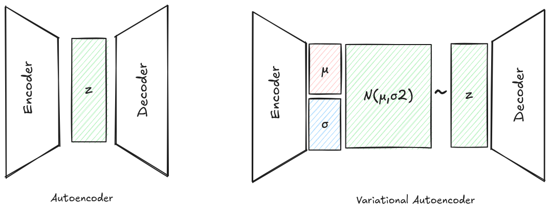
simple autoencoders are compressors. encoder maps x → z, decoder maps z → x', you train with reconstruction loss like $|x - x’|^2$. great for compression, denoising, inpainting, colorization. your phone’s image sharpening features are basically denoising autoencoders. take a clean image, add noise/blur, encode-decode, and compute loss against the clean version.

the issue comes when you want to generate something new. say you trained an autoencoder on dog images. you have a known latent vector $z_{dog}$ that decodes to a dog. now you sample some $z$ close to $z_{dog}$ and decode it. what do you get?

probably garbage. or a totally unrelated image.

reason: nothing in the loss function tells the network how to organize its latent space. the only constraint is “reconstruct well.” so the encoder dumps latent vectors wherever it wants. sparse clumps with huge empty regions in between. the latent space is full of holes. sample from a hole, get noise.

the fix: constrain the latent space

VAEs say: instead of letting the encoder map to a single deterministic point, let it map to a distribution over latents. specifically a Gaussian. and then add a loss term that pulls all those per-input Gaussians toward a standard normal $\mathcal{N}(0, I)$.

the encoder now outputs two things: $\mu_\phi(x)$ and $\sigma_\phi(x)$. you sample $z \sim \mathcal{N}(\mu, \sigma^2)$ and decode that.

the loss has two parts:

\[\begin{aligned} \mathcal{L} &= \underbrace{\mathbb{E}_{q(z \mid x)} [-\log p(x \mid z)]}_{\text{reconstruction}} \\ &\quad + \underbrace{\operatorname{KL} (q(z \mid x) \,\Vert\, p(z))}_{\text{regularization}} \end{aligned}\]

reconstruction term says “decoder should reconstruct $x$ from $z$.” KL term says “the per-input distribution shouldn’t drift too far from the prior $\mathcal{N}(0, I)$.”

intuition: the KL term forces all your encoder outputs to overlap with each other near the origin. similar inputs land in overlapping Gaussians, so interpolating in latent space gives smooth interpolation in image space. and sampling from $\mathcal{N}(0, I)$ at inference time actually lands you somewhere the decoder has seen.

but where does this loss come from?

this isn’t ad-hoc. it falls out of doing variational inference properly.

what we actually want is to model $p(x)$, the distribution over images. by marginalizing:

\[p(x) = \int p(x \mid z)\, p(z)\, dz\]

this integral is intractable for any interesting decoder $p(x \mid z)$. so we can’t directly maximize likelihood.

variational inference trick: introduce an approximate posterior $q_\phi(z \mid x)$ (this is the encoder), and use Jensen’s inequality.

\[\begin{aligned} \log p(x) &= \log \int q(z \mid x) \frac{p(x \mid z)\, p(z)}{q(z \mid x)}\, dz \\ &\geq \mathbb{E}_q\!\left[ \log \frac{p(x \mid z)\, p(z)}{q(z \mid x)} \right] \end{aligned}\]

expand the right side:

\[\begin{aligned} \log p(x) &\geq \mathbb{E}_q[\log p(x \mid z)] \\ &\quad - \operatorname{KL}(q(z \mid x) \,\Vert\, p(z)) \\ &:= \operatorname{ELBO} \end{aligned}\]

that’s the evidence lower bound. maximizing ELBO ≈ maximizing $\log p(x)$. the negative ELBO is exactly the VAE loss above.

nuance #1: ELBO is a lower bound, and the gap is meaningful

the gap between $\log p(x)$ and ELBO is not zero. it’s:

\[\log p(x) - \operatorname{ELBO} = \operatorname{KL}(q_\phi(z \mid x) \,\Vert\, p(z \mid x))\]

i.e. the KL between your approximate posterior (encoder) and the true posterior. so when you optimize ELBO, you’re simultaneously:

1. fitting the data ($\log p(x)$ goes up)
2. tightening the bound (encoder gets closer to true posterior)

this is the part that gets glossed over in most tutorials. the encoder isn’t just a feature extractor, it’s an approximation to an intractable posterior, and a bad encoder means a loose bound on likelihood. you can’t separate “good encoder” from “good likelihood model”, they’re the same optimization.

the reparameterization trick

so the loss looks fine on paper. you sample $z \sim \mathcal{N}(\mu, \sigma^2)$, compute reconstruction loss + KL, backprop.

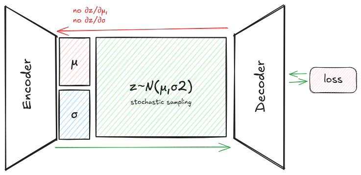
problem: you can’t backprop through sample(). sampling is stochastic. there’s no $\partial z / \partial \mu$ for “draw a sample from this distribution.”

the trick

instead of $z \sim \mathcal{N}(\mu, \sigma^2)$, write:

\[z = \mu + \sigma \odot \varepsilon, \quad \varepsilon \sim \mathcal{N}(0, I)\]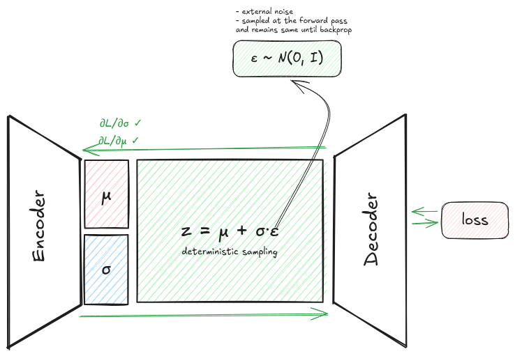

now the randomness is isolated to $\varepsilon$, which has no learnable parameters. $\mu$ and $\sigma$ are deterministic functions of $x$. gradients flow through $\mu$ and $\sigma$ as normal.

the trick works because the Gaussian belongs to the location-scale family. any Gaussian can be written as a deterministic affine transform of a standard Gaussian. this is why it doesn’t generalize trivially to e.g. a categorical distribution. that’s why VQ-VAE needs a different trick (straight-through estimator).

nuance #2: why reparam beats REINFORCE

there’s an alternative way to estimate $\nabla_\phi \mathbb{E}{q\phi}[f(z)]$: the score function estimator (REINFORCE):

\[\nabla_\phi \mathbb{E}_{q_\phi}[f(z)] = \mathbb{E}_{q_\phi}\!\left[ f(z)\, \nabla_\phi \log q_\phi(z) \right]\]

this works for any distribution, not just location-scale. but variance is brutal. reparameterization gives:

\[\begin{aligned} \nabla_\phi \mathbb{E}_{p(\varepsilon)} [f(g_\phi(\varepsilon))] &= \mathbb{E}_{p(\varepsilon)}\!\left[ \nabla_z f(z)\big|_{z=g_\phi(\varepsilon)} \cdot \nabla_\phi g_\phi(\varepsilon) \right] \end{aligned}\]

the gradient estimator now uses $\nabla_z f$, which carries way more signal than just the scalar value $f(z)$. lower variance = faster convergence. this is the reason VAEs use Gaussians (or other reparameterizable distributions) and not arbitrary priors.

nuance #3: predict log-variance, not variance

in practice the encoder predicts $\log \sigma^2$ rather than $\sigma$ or $\sigma^2$ directly. three reasons:

1. $\sigma > 0$ is a hard constraint. predict $\log \sigma^2$, exponentiate, positivity is free.
2. neural net outputs are unbounded; matching unbounded → unbounded is easier to train than unbounded → $\mathbb{R}^+$.
3. the closed-form KL has $\log \sigma^2$ in it directly (see below), so you save a log op and avoid log(0) underflow.

the KL term in closed form

for prior $p(z) = \mathcal{N}(0, I)$ and posterior $q(z \mid x) = \mathcal{N}(\mu, \sigma^2 I)$ with diagonal covariance, the KL has a clean closed form:

\[\begin{aligned} \operatorname{KL}(q \,\Vert\, p) &= \frac{1}{2} \sum_{i=1}^d \left( \mu_i^2 + \sigma_i^2 \right. \\ &\qquad\left. - \log \sigma_i^2 - 1 \right) \end{aligned}\]

no monte carlo needed for this term, it’s analytic. only the reconstruction term needs sampling. this is one of the engineering reasons everyone uses Gaussian prior + diagonal Gaussian posterior. the math is just clean.

the implicit decoder distribution (a thing nobody tells you)

look at most VAE code. the reconstruction loss is MSE(x, decoder(z)). but the ELBO has $\mathbb{E}_q[-\log p(x \mid z)]$. how does MSE come from a log-likelihood?

answer: when you use MSE, you’re implicitly assuming:

\[p(x \mid z) = \mathcal{N}(x;\, \operatorname{decoder}(z),\, \sigma_x^2 I)\]

with fixed scalar variance $\sigma_x^2$. then:

\[\begin{aligned} -\log p(x \mid z) &= \frac{1}{2\sigma_x^2} \|x - \operatorname{decoder}(z)\|^2 \\ &\quad + \text{const} \end{aligned}\]

the $\sigma_x^2$ acts as a relative weight between reconstruction and KL. and this is exactly where $\beta$-VAE comes from. $\beta$ is just $\sigma_x^2$ in disguise.

if you use BCE loss, you’re assuming a Bernoulli decoder. for natural images, neither assumption is great, which is why modern “VAEs” (the ones in stable diffusion etc.) ditch this entirely and use perceptual loss + GAN loss + tiny KL regularizer. more on this below.

things nobody tells you

the hole problem

we want sampling at inference to work: $z \sim p(z) = \mathcal{N}(0, I)$, then decoder(z) should give a reasonable image. for this to work, the aggregated posterior

\[q(z) = \mathbb{E}_{x \sim p_{\text{data}}} [q(z \mid x)]\]

should match $p(z)$. but the KL term in ELBO only minimizes per-input $\operatorname{KL}(q(z \mid x) \,\Vert\, p(z))$, it doesn’t directly enforce the aggregated thing.

result: $q(z) \neq p(z)$ in general. there are regions of latent space that have prior mass but no encoder ever mapped to. when you sample there, you get garbage. these are the “holes.”

this is the reason VAE samples look blurry/weird relative to GAN or diffusion samples. it’s not a decoder capacity issue. it’s a marginal mismatch issue. the encoder paints inside the lines but doesn’t fill the canvas.

fixes that work to varying degrees: VampPrior (use a learnable mixture of $q(z \mid x_k)$ as the prior), normalizing flow priors, hierarchical VAEs (NVAE, VDVAE).

posterior collapse

if your decoder is powerful enough to model $p(x)$ on its own (e.g. autoregressive decoder for text/audio), the optimizer finds a cheap local minimum: set $q(z \mid x) = p(z)$ for all $x$. KL term goes to zero. decoder ignores $z$ entirely.

congrats, you trained an unconditional model with extra steps.

most common in NLP VAEs with LSTM/transformer decoders. fixes:

• KL annealing: start with $\beta = 0$, ramp up over training. lets reconstruction win first.
• free bits: allow KL to be “free” up to some threshold per dimension. clamp via $\max(\lambda, \text{KL})$ instead of $\text{KL}$.
• bottleneck the decoder: weaker decoder = more pressure on $z$ to carry info.

this is the part that bites you hardest if you naively try to put a VAE on top of a transformer text decoder.

the rate-distortion view ($\beta$-VAE)

rewrite the loss with explicit weight:

\[\begin{aligned} \mathcal{L} &= D + \beta R \\ D &= \mathbb{E}_q[-\log p(x \mid z)] \\ R &= \operatorname{KL}(q(z \mid x) \,\Vert\, p(z)) \end{aligned}\]

this is literally the rate-distortion lagrangian from information theory. the VAE is a lossy compressor with rate $R$ (bits used to encode $z$) and distortion $D$ (reconstruction error). $\beta$ controls the tradeoff:

• $\beta \to 0$: pure autoencoder. rate is unbounded, distortion → 0.
• $\beta = 1$: standard VAE.
• $\beta > 1$: $\beta$-VAE. forces disentangled / low-rate representations.

every VAE you’ve ever seen sits somewhere on this rate-distortion curve. the choice of $\beta$ is a choice of operating point on a tradeoff, not a hyperparameter to “tune for best results.” there’s no objectively best $\beta$, only different points on the frontier.

the linear-Gaussian case is just probabilistic PCA

if encoder and decoder are linear and the decoder noise is isotropic Gaussian, VAE reduces to probabilistic PCA (Tipping & Bishop, 1999). the latent dimensions align with principal components.

so VAE is the nonlinear extension of pPCA. useful sanity check: your fancy nonlinear VAE should at minimum do something sensible on linear-Gaussian data, which means it should recover pPCA.

the “VAE” in stable diffusion is barely a VAE

LDM’s first-stage model is trained with:

• L1 reconstruction loss (not MSE)
• LPIPS perceptual loss (deep feature distance)
• patchgan adversarial loss
• KL regularization with $\beta$ on the order of $10^{-6}$

the KL term is so small it barely does anything. the latent space is regularized mostly by the perceptual + GAN losses, not by the prior. people call it a VAE for historical reasons but it’s really a KL-regularized autoencoder, sometimes labeled “KL-AE” in the literature.

the alternative first stage in LDM is VQ-GAN. also called a “VQ-VAE” in casual usage even though, again, it’s heavily GAN-trained and uses straight-through estimators rather than reparameterization.

moral: when someone says “VAE” in 2026, ask which loss terms they’re actually using.

where VAEs actually live today

short version of the modern usage map:

• latent diffusion: stable diffusion, SDXL, SD3, flux. all run diffusion in a (KL+GAN+perceptual)-trained autoencoder latent. video diffusion (sora, hunyuan, cogvideox, wan) extends this with 3D causal VAEs that compress space and time.
• discrete tokenizers for autoregressive multimodal: VQ-VAE, VQ-GAN, MAGVIT-v2 with LFQ, FSQ. used in muse, parti, llamagen, emu3, unified vision-language models.
• neural audio codecs: SNAC, mimi, encodec, DAC. all are RVQ-VAEs (residual vector quantization). modern TTS (CSM-1B, maya, etc.) depends on these to tokenize audio for an LM head.
• world models: dreamerv3, genie. VAE-style encoders compress observations into a latent space where a small recurrent dynamics model can plan.
• scientific ML: scVI / scANVI for single-cell RNA-seq. one of the few places where the probabilistic interpretation actually buys you something. you need calibrated uncertainty over count distributions and the ELBO machinery handles that natively.

what died: VAEs as standalone image generators (GANs and diffusion crushed them on FID), and VAEs as the primary tool for image SSL (MAE, DINO/DINOv2, SigLIP variants dominate now).

through-line: VAE-the-architecture-pattern is everywhere. VAE-the-probabilistic-purist-method mostly lives on in scientific applications and as a footnote in deep learning history.

---